Volatility Modeling of U.S. 10-Year Treasury Yields Using GARCH
This page presents a GARCH (Generalized Autoregressive Conditional Heteroskedasticity) volatility analysis of 10-Year U.S. Treasury yields using data from the Federal Reserve Economic Data (FRED).
Summary Statistics
Key statistics for 10-Year Treasury yields and their daily changes over the analysis period (1990-2025).
| Statistic | Value |
|---|---|
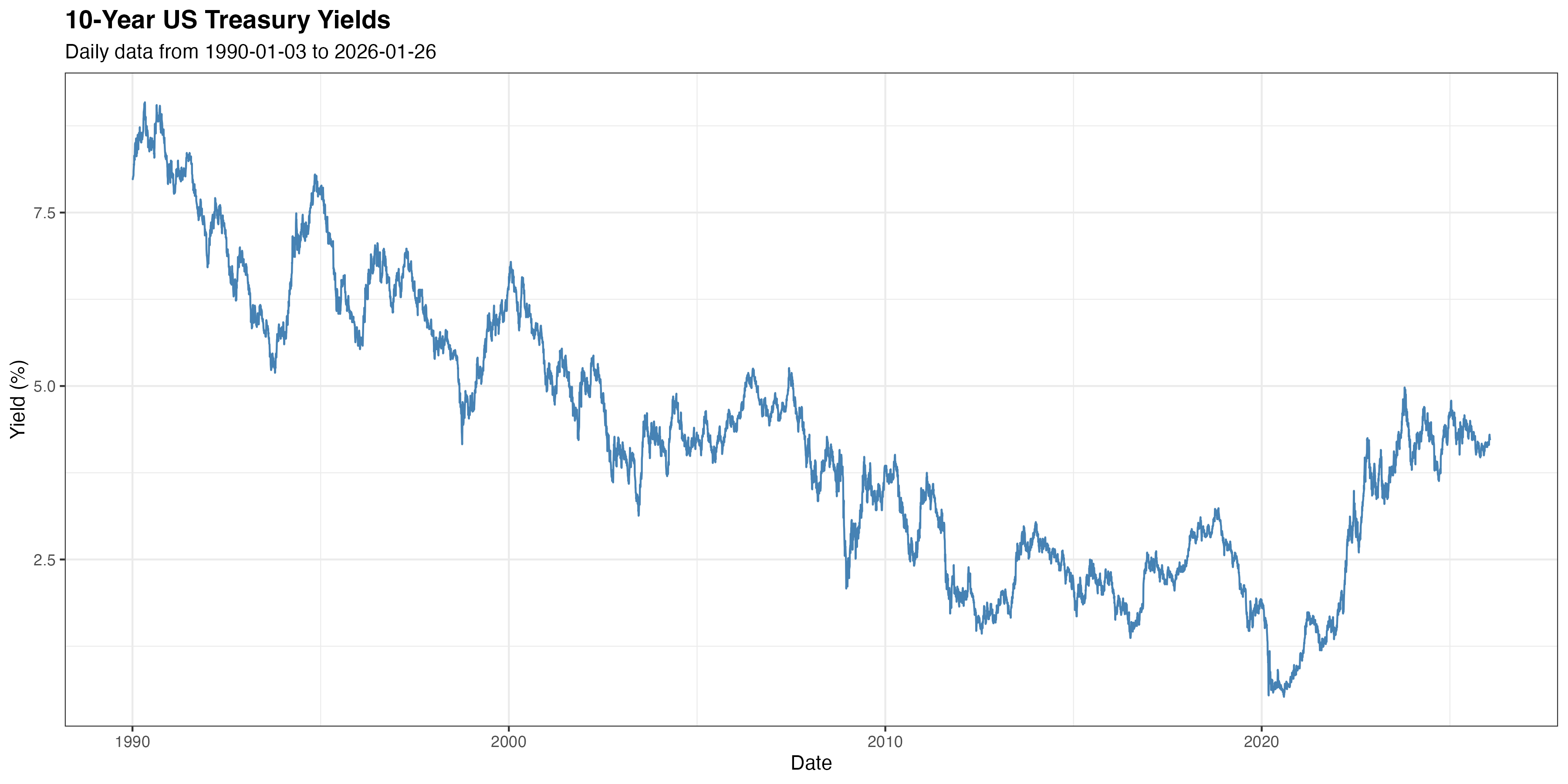
| Mean Yield | 4.26% |
| Median Yield | 4.17% |
| Std Dev of Yield | 1.94% |
| Min Yield | 0.52% |
| Max Yield | 9.09% |
| Mean Daily Change | -0.0004 pp |
| Std Dev of Daily Change | 0.069 pp |
| Skewness | 0.044 |
| Kurtosis | 5.44 |
Key Observations:
- Average 10-year yield over the period: 4.26%
- High kurtosis (5.44) indicates fat tails - extreme yield changes occur more frequently than a normal distribution would predict
- Near-zero skewness (0.044) suggests relatively symmetric distribution of changes
1. Historical 10-Year Treasury Yields
The complete time series of 10-Year U.S. Treasury constant maturity rates.
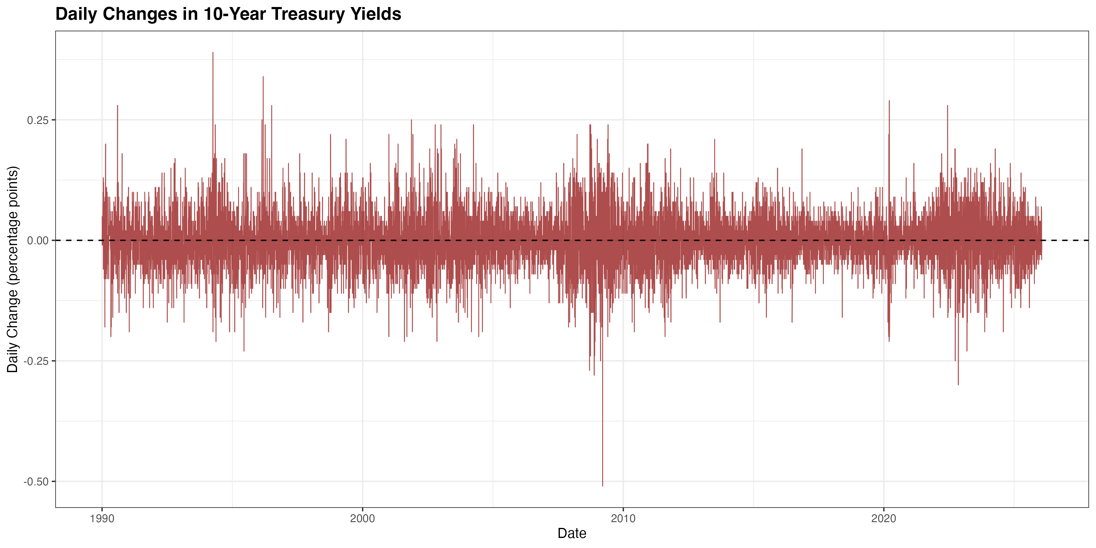
2. Daily Yield Changes
Daily changes in Treasury yields show periods of high and low volatility, with occasional extreme movements during market stress events.
3. Distribution of Yield Changes
The distribution of daily yield changes compared to a normal distribution (red dashed line).

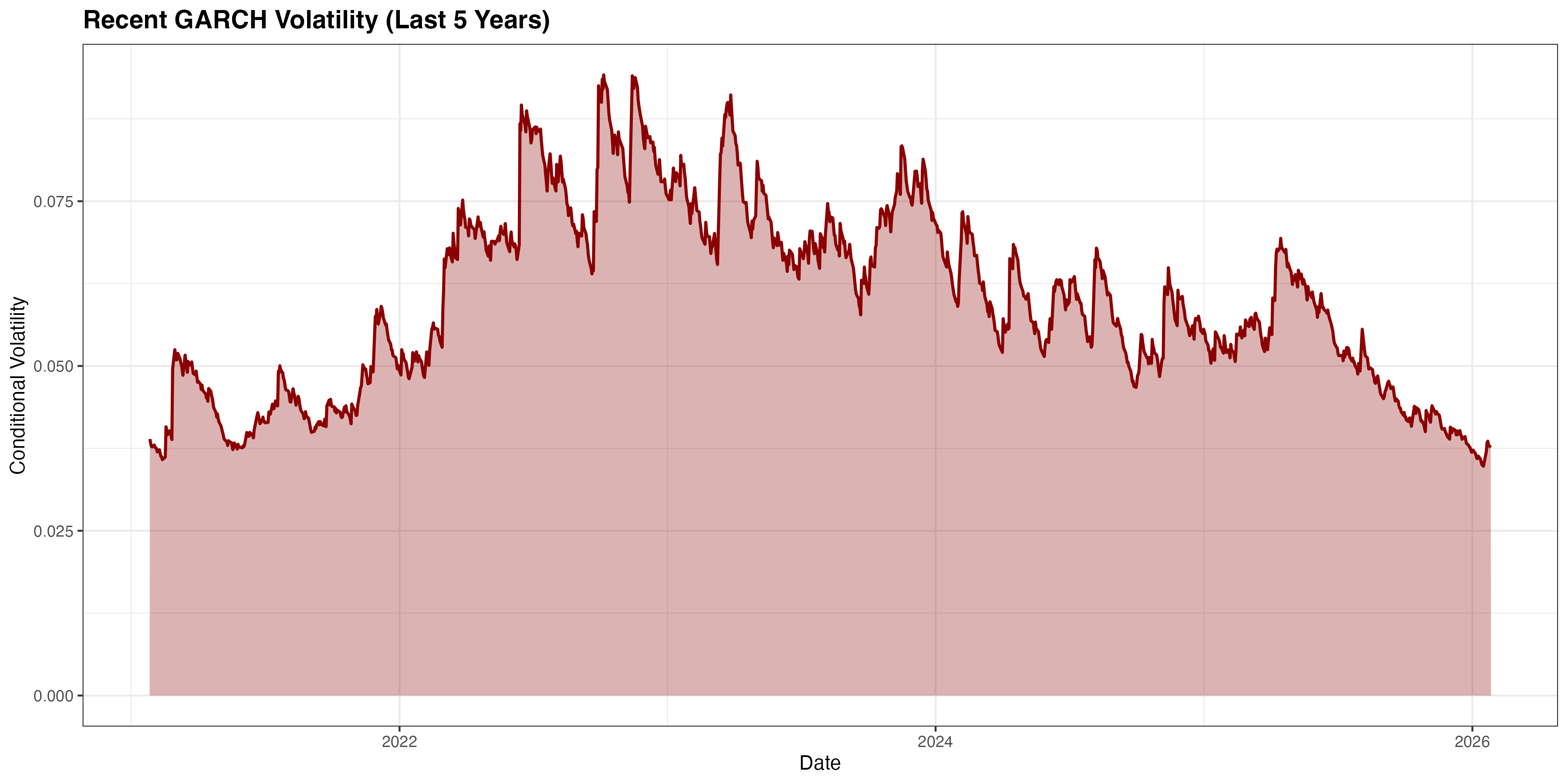
4. GARCH(1,1) Conditional Volatility
The estimated volatility from the GARCH(1,1) model. This represents the model’s real-time estimate of the standard deviation of yield changes.
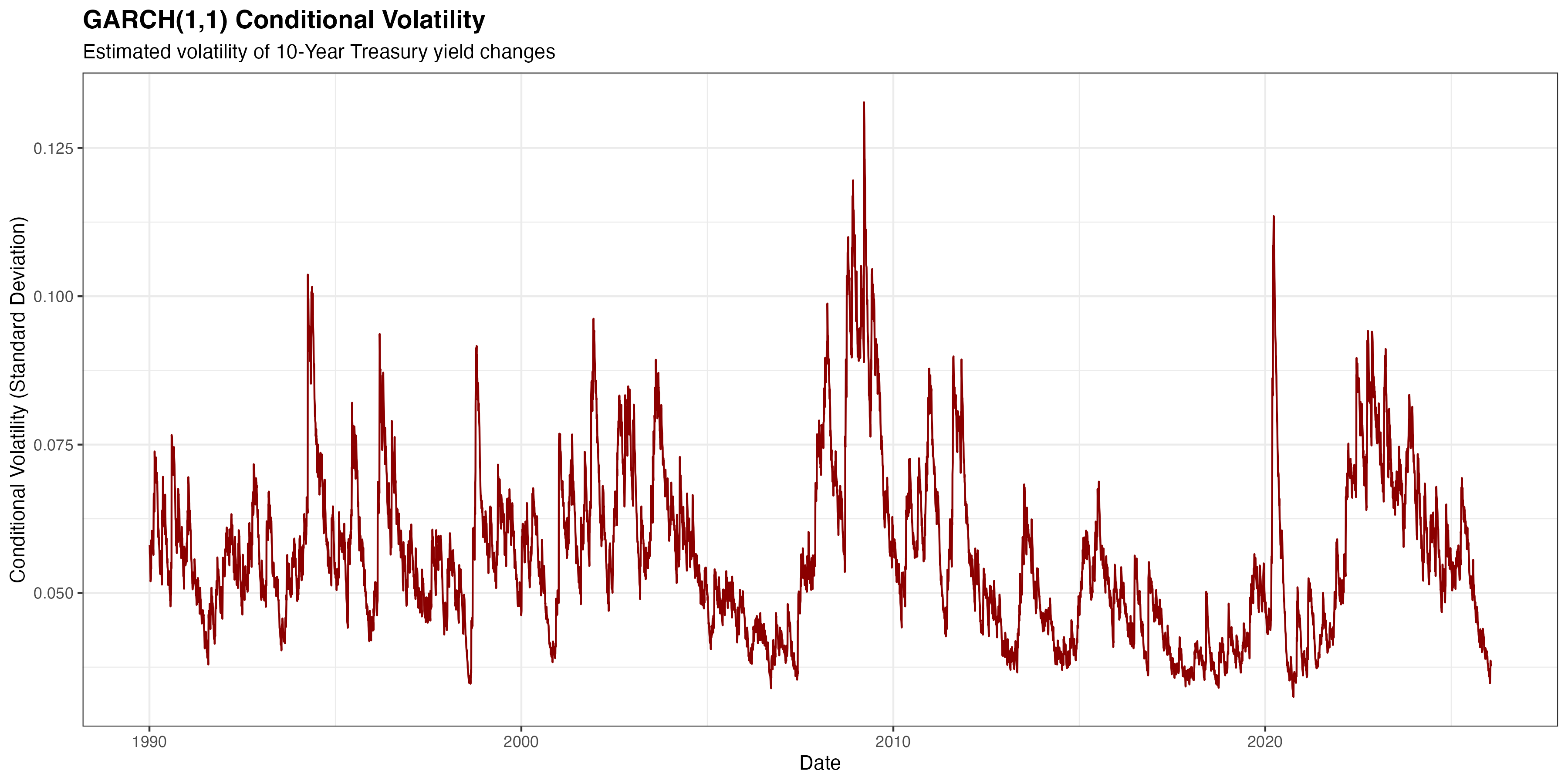
Key observations:
- Volatility spikes during financial crises and market stress
- Clear evidence of volatility clustering
- Volatility is time-varying and persistent
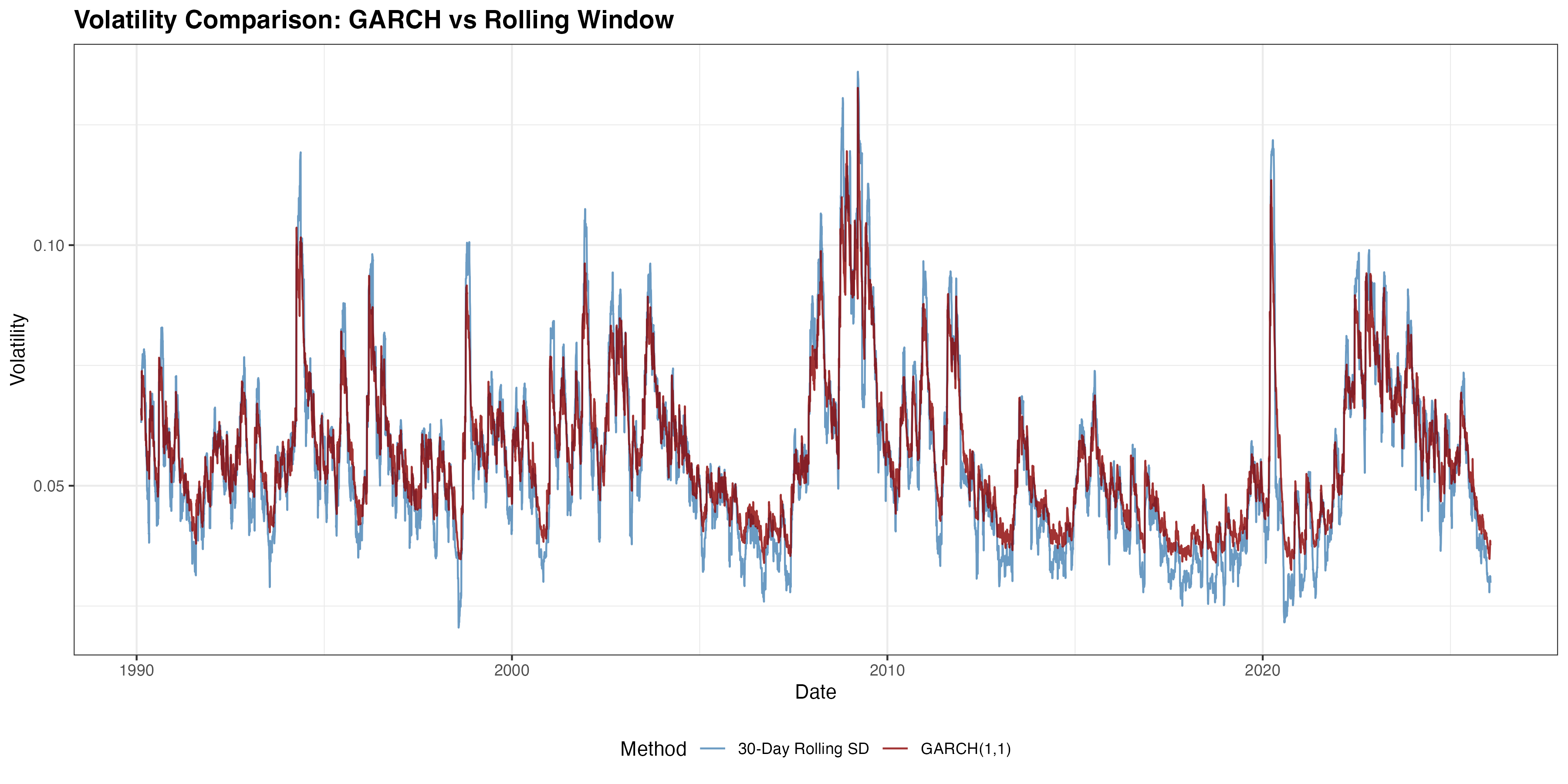
5. GARCH vs Rolling Window Volatility
Comparison between GARCH(1,1) conditional volatility and a simple 30-day rolling standard deviation.
6. Recent Volatility (Last 5 Years)
7. Evidence of Volatility Clustering
Autocorrelation function (ACF) of squared yield changes. Significant autocorrelation indicates volatility clustering.
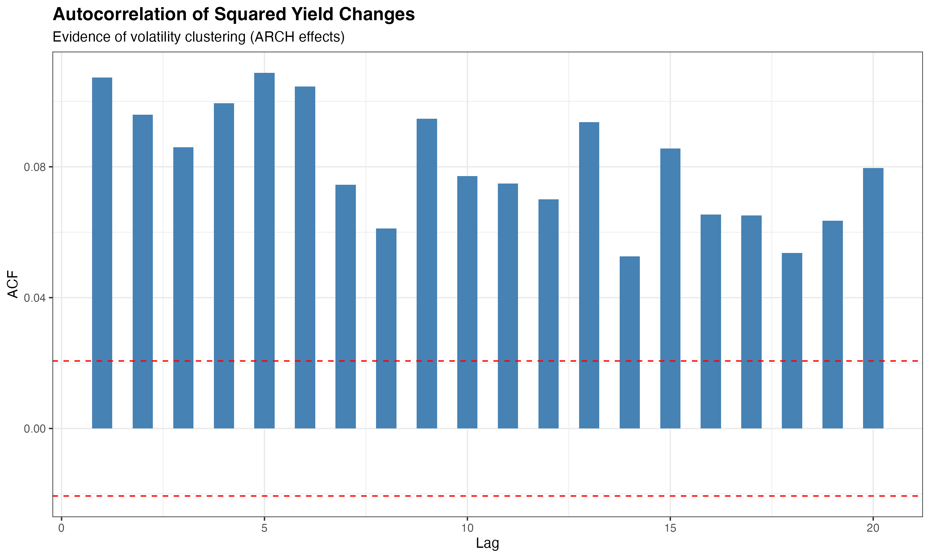
Bars extending beyond the red dashed lines indicate statistically significant autocorrelation, confirming the presence of ARCH effects (volatility clustering).
GARCH Model Results
Model Specification
- Model: GARCH(1,1)
- Mean equation: Constant mean
- Variance equation: σ²ₜ = ω + α·ε²ₜ₋₁ + β·σ²ₜ₋₁
Where:
- ω (omega): Long-run variance level
- α (alpha): Impact of past shocks on current volatility
- β (beta): Persistence of volatility
- α + β: Total persistence (closer to 1 = more persistent)
Model Comparison
Two GARCH(1,1) models were estimated:
- GARCH(1,1) with Normal distribution
- GARCH(1,1) with Student-t distribution
Interpretation
What does this analysis tell us?
- Volatility is not constant: Treasury yield volatility varies significantly over time
- Volatility clusters: High volatility periods are followed by high volatility, low by low
- Persistence: Volatility shocks have long-lasting effects
- Predictability: GARCH models can forecast near-term volatility with reasonable accuracy
Methodology
Data Source
- 10-Year Treasury Constant Maturity Rate (DGS10) from FRED
- Daily frequency
- Starting from 1990 (adjustable)
Software & Packages
Analysis performed in R using:
quantmod: Data download from FREDrugarch: GARCH model estimationtidyverse: Data manipulation and visualizationforecast: Time series analysis
Model Diagnostics
The analysis includes:
- Ljung-Box test for ARCH effects
- Information criteria (AIC, BIC) for model comparison
- ACF plots for volatility clustering
- Standardized residuals analysis
Files Available for Download
After running the analysis, the following CSV files are generated:
Treasury_10Y_GARCH_Analysis.csv- Full dataset with yields and volatility estimatesGARCH_Coefficients.csv- Estimated model parametersGARCH_Model_Comparison.csv- Model selection criteriaSummary_Statistics.csv- Descriptive statistics